Energy Based Models
From basics to LLMs
Transformers are already
energy-based models
We just don't see them that way (yet)
Three recent results
🏆 55M-parameter energy-based reward model
127× smaller than typical reward models — boosts Llama 3 to 90.7% on GSM8k, 63.7% on MATH
Jiang et al, Learning to Rank Chain-of-Thought, 2025
📈 Energy-based Transformers scale 35–57% faster
Better data efficiency than standard autoregressive transformers, tested up to 120B tokens
Gladstone et al, Energy-Based Transformers are Scalable Learners and Thinkers, 2025
🎯 RLHF optimal policy = Boltzmann distribution
The optimal policy in RLHF is literally the Boltzmann distribution over reward-weighted outputs
Talk outline
1. The Energy-Based Model paradigm
2. How do we train EBMs?
3. EBMs meet LLMs
Part 1
The Energy-Based
Model Paradigm
The Energy Landscape
- Blue = low energy ≈ good
- Red = high energy ≈ bad
- Training = shaping the landscape
- Inference = rolling a ball downhill
The Energy Function
The energy function is the model. It maps every possible configuration x to a scalar — shaping the landscape you just saw.
⬇️
Low energy = "looks like real data"
⬆️
High energy = "doesn't look like data"
Unlike a loss function (a training-time objective over θ), the energy function defines the model itself — any function is valid. No normalization constraints, no factorization required.
The Compatibility View
More generally, given an input x and a candidate answer y, the energy function returns "how incompatible are they?"
⬆️
High energy = incompatible
⬇️
Low energy = compatible
"Probability comes at a high price, and should be avoided when the application does not require it" — Yann LeCun
Inference
Find Y that minimizes E
- Inference is now an optimization problem
- No sampling, no autoregressive decoding, no beam search
Energy-Based vs. Autoregressive
Energy–Probability Duality
The Boltzmann Distribution
From the maximum entropy principle: among all distributions consistent with a given average energy, the Boltzmann distribution has the maximum entropy.
Key insight: probability ratios are energy differences → independent energy functions combine additively
Temperature as a Sharpness Control
Temperature controls how peaked vs. flat the probability distribution is.
- Low T → sharp peaks (deterministic)
- High T → flat (exploratory)
Connection to Transformer Decoding
When a transformer produces logits over the vocabulary and you compute , you are treating the negative logits as an energy function over vocabulary items and computing the Boltzmann distribution at temperature T.
"I set temperature to 0.3" → more deterministic output
"I set temperature to 1.5" → more creative output
They are adjusting the Boltzmann temperature of an energy-based model.
The Partition Function (Problem)
Sum (or integral) over all possible configurations X
🖼️ Images (256×256×3, 8-bit)
256^(256×256×3) ≈ 10^473,000
📝 Text (length 1000, vocab 50k)
50,000^1000
The intractable partition function was one reason EBMs fell out of fashion. We will revisit it in a moment.
Likelihood Estimation
Train the EBM by minimizing the negative log-likelihood:
Step 1 — Expand the NLL
Step 2 — Take the gradient w.r.t. θ
Step 3 — The key identity:
Combining steps 2 and 3:
Two-Phase Training
Positive Phase
Push energy down on real data
Just requires a dataset — tractable
Negative Phase
Push energy up on model samples
Requires sampling from — the hard part
Without the negative phase, the model assigns low energy everywhere — it learns "real data is good" but never learns what is bad.
The gradient is independent of — but sampling from is not!
Positive Phase
Push energy DOWN on real data.
The expectation is on the data distribution — picking samples from our dataset. The update changes parameters to minimize the energy at data points.
Negative Phase
Push energy UP on model samples.
We sample from — the model's current distribution. These are points where the model has placed high probability (low energy). The update raises energy on these points, eroding misallocated probability mass.
Combined with the positive phase, the effect is: keep probability on real data, remove it from everywhere else.
Two-Phase Training Demo
Why Both Phases Matter
Positive phase alone
Simple gradient descent on data — tractable.
But leads to degenerate solutions: the model could assign constant energy everywhere.
Model learned "real data is good" but never learned what is bad.
Negative phase is essential
Provides contrast — teaches the model what doesn't look like data by pushing energy up on incorrect configurations.
But sampling from is intractable in high dimensions — this is where the difficulty comes from.
Recap
An EBM is a scoring function . Low = good.
Probabilities require the partition function Z, which is intractable. Avoid computing it.
Training requires both pushing energy down on data AND pushing energy up on wrong answers.
Up Next
How to train your EBM? — Contrastive divergence, score matching, noise-contrastive estimation, and more.
Part 2
How to Train
Your EBM
Based on Song & Kingma, "How to Train Your Energy-Based Models" (2021)
The core challenge
We derived the gradient of the negative log-likelihood:
But the negative phase requires sampling from:
where is intractable for large dimensions. So how do we handle this?
Three approaches
1. Markov Chain Monte Carlo
Generate negative samples by running a Markov chain
2. Score Matching
Avoid sampling altogether — match the gradient of the log-density
3. Noise Contrastive Estimation
Cast density estimation as binary classification (data vs. noise)
Approach 1
Markov Chain
Monte Carlo
MCMC: The Idea
Can't sample from exactly — the partition function blocks us.
But we can approximately sample by running a Markov chain that converges to in the limit.
💡 Key insight
Run an MCMC sampler to generate approximate negative samples x⁻, then plug them into the gradient equation as if they were exact samples from .
The score doesn't need Z — so gradient-based MCMC is feasible!
Langevin Dynamics
Starting from a random point, iteratively follow the energy gradient with noise:
- is the current position in configuration space
- moves toward lower energy (the signal)
- adds stochastic exploration (the noise)
When ε → 0 and K → ∞, is guaranteed to distribute as under regularity conditions.
MCMC + Gradient Update
Once we have Langevin samples, plug them into the two-phase gradient:
Data samples (minibatch)
Langevin samples (MCMC)
The Problem with MCMC
Langevin dynamics can take a very long time to converge, especially in high-dimensional spaces with multiple modes.
If we need 10,000 Langevin steps per sample, and we need samples for every gradient update during training, the whole thing is prohibitively slow.
The mixing problem
If the energy landscape has widely separated modes with high-energy barriers, the chain gets trapped in one mode. The negative samples only represent that region, leaving other modes untouched. This gets worse in high dimensions.
Hack: Contrastive Divergence
Hinton, 2002
Don't start the chain from a random point — start from a data point.
CD-1: One MCMC step from data
Very biased, doesn't represent true MLE — but works surprisingly well in practice.
Persistent CD (Tieleman 2008)
Don't reset the chain between updates — carry over the state. Works because model parameters change slowly between updates.
Replay Buffer (Du & Mordatch 2019)
Keep historical MCMC states in a buffer, randomly sample to initialize new chains.
MCMC Sampling Demo
Approach 2
Score Matching
Reformulate learning to avoid sampling altogether
The Score Function
The score of a distribution is the gradient of the log of probability density with respect to the input:
For an EBM with :
log Z_θ vanishes! — because Z_θ is a constant with respect to x. The score only depends on the energy function, not the intractable partition function.
Why Scores Are Enough
If two continuously differentiable log probability density functions (PDFs) have equal first derivatives everywhere, and both integrate to 1, they must be the same distribution.
So we can learn the right distribution by matching scores rather than matching probabilities:
No partition function, no sampling, no MCMC — just make the model's score look like the data's score.
Fisher Divergence
Formally, minimize the Fisher divergence between model and data scores:
where the scores are gradients of log probability densities:
Expanding the squared norm:
Problem: the cross-term contains — we don't know , only samples from it!
Integration by Parts Trick
Hyvärinen (2005) showed the Fisher divergence can be rewritten using only the model's score and its Jacobian:
We only need the model's score and its Jacobian (the Hessian of ).
But: the trace requires second-order derivatives — O(d) backward passes for dimensionality d. Computationally infeasible for high dimensions.
Denoising Score Matching
Vincent, 2011
Instead of matching scores on clean data (which requires the Hessian), corrupt data with noise: , where .
The noise kernel is a known Gaussian, so its score has a simple closed form:
Now match the model's score to this known target:
No second-order derivatives, no unknown — just a regression problem: predict the noise direction from the noisy input.
Diffusion Models from the EBM Lens
If we perform denoising score matching at many noise levels — from pure noise down to near-zero noise — we get a multi-scale score model.
Sample by starting from noise and gradually denoising via Langevin dynamics at decreasing noise scales (annealed Langevin dynamics).
Takeaway
Denoising score matching ≡ denoising diffusion probabilistic models, just viewed through different lenses (score vs. probability).
Diffusion models are EBMs trained via denoising score matching.
Song & Ermon 2019; Ho et al. 2020; Song et al. 2021
Approach 3
Noise Contrastive
Estimation
Cast density estimation as binary classification
NCE: The Idea
No more trying to sample from or match its score.
Instead, train a binary classifier to tell whether a sample came from the data distribution or a known noise distribution.
Any classifier that can answer this optimally can implicitly recover the data density — this is theoretically proven (Gutmann & Hyvärinen, 2010).
Unique advantage: NCE learns Z as a by-product — the only method among the three that does.
NCE: Two Sources
1. Data distribution
Can sample from training set.
2. Noise distribution
Could be Gaussian, uniform, or… the output of a pretrained autoregressive model 🧐
(spoiler alert)
Must be able to both sample from and evaluate its density at any point.
Mix them together: draw x from either source with equal probability, then ask the classifier: "which source did this come from?"
NCE: At Optimality
At optimality, the classifier's posterior matches the true posterior:
When the classifier is optimal, — the model has recovered the data distribution.
NCE defines , making the log-normalizer a learnable scalar optimized jointly with θ. At convergence, c → −log . This is the only training paradigm among the three that actually recovers Z.
NCE: The Objective
The NCE loss is a binary cross-entropy — classify each sample as data or noise:
This serves as our training loss for the EBM: the energy function is updated so that the model assigns high density to data samples and low density to noise samples — the positive and negative phases emerge naturally from the two cross-entropy terms.
No MCMC sampling, no Hessian, no score functions — just a classifier and a good noise distribution.
Why Hard Negatives Matter
The closer the noise distribution is to the data distribution, the better representations are needed to distinguish them.
🎯
Easy noise (e.g. uniform)
Trivial to classify → model learns superficial features
🔥
Hard noise (e.g. pretrained LM)
Hard to classify → model must learn deep structure
This principle connects to contrastive learning broadly — SimCLR, CLIP, and ELECTRA all benefit from harder negatives.
Comparing Training Paradigms
Part 2 Recap
MCMC: Sample negatives via Langevin dynamics. Practical with contrastive divergence, but biased and struggles with high-dimensional multimodal landscapes.
Score Matching: Match ∇ₓ log p, bypassing Z entirely. Denoising variant avoids expensive Hessians and connects directly to diffusion models.
NCE: Learn density by classifying data vs. noise. The only method that learns Z. Quality depends heavily on the noise distribution.
Key theme
All three methods find creative ways to avoid the intractable partition function — MCMC sidesteps it with sampling, SM removes it via calculus, NCE absorbs it into a classifier.
Part 3
EBMs 🤝 LLMs
Your Classifier Is Secretly an EBM
Grathwohl et al., JEM, 2020
A standard classifier with softmax:
There is a hidden energy-based generative model inside every discriminative classifier.
The JEM Reinterpretation
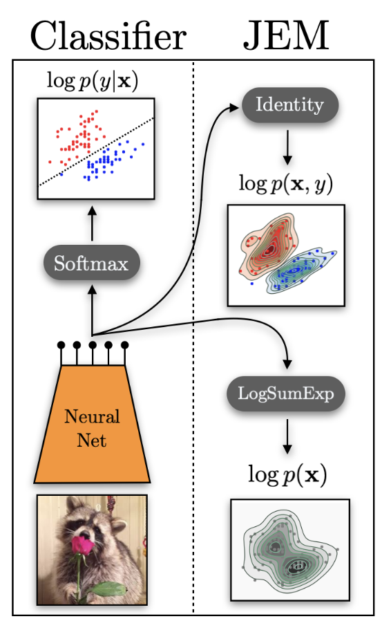
Reinterpret the logits as a joint energy function:
Here — normalizing over all (x, y) pairs introduces the intractable EBM partition function.
Marginalize out y to get an energy over inputs:
The same neural net logits which we used to define the discriminative p(y|x) can be used to define the joint p(x, y) and the generative p(x).
Training the Joint EBM
Decompose the joint log-probability:
— generative term
Trained via SGLD (Langevin dynamics)
— discriminative term
Standard cross-entropy loss
Results (all comparisons on the same WideResNet architecture and CIFAR datasets):
- Better classification than a discriminative-only model trained with the same architecture
- Better generation (FID scores) than generative-only baselines (Glow, flow models) on the same data
- Improved calibration — model confidence better reflects actual accuracy
- Strong out-of-distribution detection via the energy function as an OOD score
- Better adversarial robustness — the generative term acts as an implicit regularizer
ELECTRA
Pre-Training Text Encoders as Discriminators
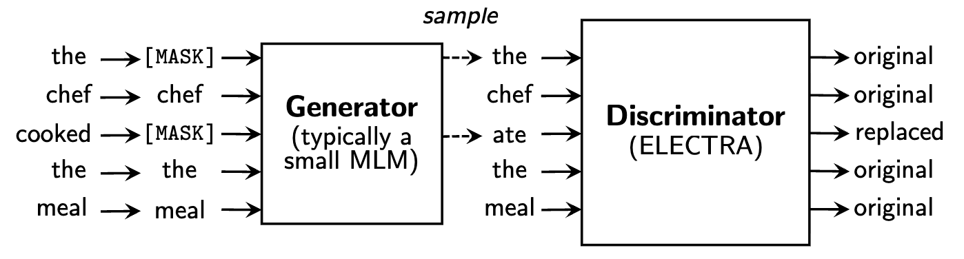
A small generator (MLM) fills in masked tokens. A larger discriminator classifies each token as original or replaced.
Why it's better than BERT MLM
- Dense signal over all tokens (not just ~15% masked)
- No [MASK] token mismatch between pre-training and fine-tuning
- 3–7× sample efficiency over BERT
ELECTRA: The EBM Connection
ELECTRA's discriminator is doing negative sampling — distinguishing real tokens (data) from fake tokens (generator output).
This is NCE with the generator as the noise distribution!
- Data distribution = real tokens from the corpus
- Noise distribution = tokens produced by the small MLM generator
- Classifier = the ELECTRA discriminator (the model we actually keep)
The generator provides hard negatives — replaced tokens that are plausible in context, forcing the discriminator to learn deep linguistic structure rather than superficial cues. This is exactly the hard negatives principle from the NCE slides.
Electric: Energy-Based Cloze Models
Clark et al., 2020
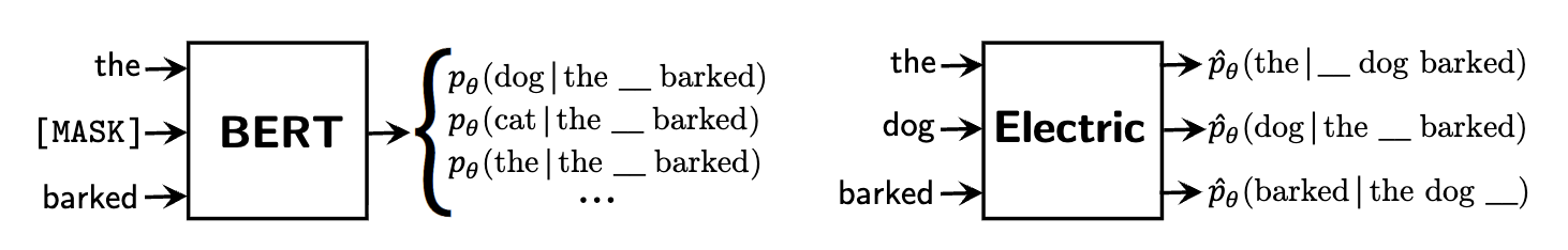
BERT predicts a distribution over the vocabulary at masked positions — it only learns from ~15% of tokens per example.
Electric outputs a cloze probability for every token given its context — how likely is this specific token in this position?
Electric produces — a scalar score per token, not a distribution over the vocabulary. Dense signal from every token, no [MASK] needed.
Electric: From Classification to Density
Electric takes ELECTRA's insight further — from binary classification to proper noise contrastive estimation:
ELECTRA
Binary classifier: "real or replaced?" Useful representations, but the output is just a label — no density estimate.
Electric
Full NCE: uses the generator's known density to convert the discriminator output into calibrated per-token pseudo-probabilities.
Because Electric models per-token cloze probabilities (not a joint sequence probability), it avoids autoregressive factorization entirely — each token is scored independently given context, making it a true energy-based model over token configurations.
Residual EBMs for Text
Deng et al., 2020
Take a pretrained autoregressive LM and multiply its distribution by an energy correction from a bidirectional model:
🔄
AR model handles fluency and local coherence (token-by-token)
🌐
Bidirectional energy provides global, sequence-level quality correction
💡 Energy-based models as "verifiers" — the EBM doesn't generate, it scores and corrects. Trained end-to-end via NCE.
EDLM: The Problem with Parallel Text Generation
Zhao et al., 2025
Discrete diffusion models for text unmask tokens in parallel, but predict each token independently:
At each denoising step, the model predicts a clean token at every masked position conditioned only on the noisy context — it cannot capture inter-token dependencies within the same prediction step.
The more parallel the model tries to be (fewer denoising steps), the worse this factorization error gets. This is the fundamental gap between diffusion and AR quality for language.
EDLM: Residual Energy Correction
Apply the residual EBM idea at every denoising step:
Two ways to get the energy function:
EDLM-AR
Plug in a pretrained AR model as the energy. Turns into parallel sampling from an AR model via importance weighting. One AR forward pass scores a complete sequence.
EDLM-NCE
Train a small energy head via NCE on top of the diffusion model. Positives = clean data, negatives = diffusion model's own predictions.
EDLM: Results
Inference: draw k candidates from diffusion model, score with energy, resample via importance weights.
Key finding
Correction matters most in early denoising steps (high masking ratio → worst factorization error). Apply importance sampling only for t ∈ [0.8, 1.0] to get most benefit at a fraction of the cost.
49%
generative perplexity improvement
1.3×
sampling speedup at same quality
400k
fine-tuning steps (NCE variant)
First diffusion model to seriously challenge autoregressive quality on language.
Energy-Based Transformers
Gladstone et al., 2025 — A radically different paradigm
Unlike EDLM which adds an energy correction, EBT makes the entire model an energy function:
Inference = gradient descent from random noise to a converged prediction:
Each gradient step is one unit of thinking. The model is simultaneously a generator (via energy minimization) and a verifier (via the energy scalar) — unified in a single model.
Three Facets of System 2 Thinking
🎯 Dynamic Compute
Iterate more on harder predictions. Same compute for "the" as "serendipitous"? Not anymore.
📊 Uncertainty
Energy at convergence directly quantifies confidence. Easy tokens → low energy. Hard tokens → high energy.
✅ Verification
Best-of-N sampling without a separate reward model. The energy IS the verifier.
All three emerge from unsupervised pretraining — no RL, no verifiable rewards.
EBT: Scaling Results
35%
faster scaling on data
28%
faster on batch size
57%
faster on depth
29%
inference improvement via thinking
First architecture to out-scale Transformer++ across multiple axes simultaneously (data, batch size, parameters, FLOPs, depth).
The P vs NP intuition
Despite slightly worse pretraining perplexity, EBTs beat Transformer++ on downstream tasks. Verification generalizes better than generation — learning to score is easier than learning to produce.
Thinking at Inference Time
EBTs can improve by using more forward passes — Transformer++ cannot.
OOD thinking boost
As data becomes more out-of-distribution, thinking helps more — roughly linear relationship. Just like humans engage deliberate reasoning for unfamiliar problems.
Thinking scales with training
As the model sees more data, the benefit from self-verification increases from 4–8% → 10–14%. Extrapolation to Llama-3 scale suggests potentially massive gains.
Current limitations
Experiments up to 800M parameters. Training overhead 3.3–6.6×. Struggles with multi-modal distributions (merges nearby modes). Open question: do advantages persist at GPT-4 scale?
Further Reading
ARMs are Secretly EBMs
Blondel, Sander, Vivier-Ardisson, Liu, Roulet (Google DeepMind, 2025)
Establishes an exact bijection between autoregressive models and EBMs via the chain rule of probability. Shows this corresponds to the soft Bellman equation in MaxEnt RL — giving a formal justification for why next-token predictors can plan ahead.
Continuous Autoregressive Language Models (CALM)
Phan, Tschannen, Grathwohl, et al. (Google DeepMind, 2025)
Replaces the discrete softmax head with an energy-based generative head that predicts continuous vectors. Predicts K tokens at once via a lightweight residual MLP, using energy minimization instead of categorical sampling.
EORM: Energy Outcome Reward Model
Jiang, Luo, Pang, et al. (UCLA, 2025)
A 55M-parameter energy-based reward model that ranks Chain-of-Thought solutions — 127× smaller than typical reward models. Boosts Llama 3 8B to 90.7% on GSM8k by selecting the best reasoning path via energy scoring.
The Spectrum of Energy-Based LLMs
Conservative: EBM as correction layer
JEM, Electric, Residual EBMs, EDLM, EORM — keep existing models, add energy-based scoring on top. Practical, already works at scale.
Radical: EBM as the whole model
EBTs, CALM — the transformer IS the energy function, or uses an energy-based generative head. Theoretically cleaner, remarkable scaling, built-in verification.
Unifying: ARMs ≡ EBMs
Blondel et al. show every autoregressive model has an equivalent EBM via the chain rule — the distinction is less about architecture and more about how we train and decode.
Four Takeaways
1. Verification scales better than generation
EBT shows learning an energy function (verifier) scales 35–57% faster than a feed-forward predictor. Scoring is easier than producing.
2. Test-time compute has a principled framework
Energy minimization: each gradient step = one thinking step, energy = confidence, convergence = stopping criterion. No ad-hoc prompting tricks needed.
3. Composition is the killer feature
Additive energy functions give modular, tunable, interpretable control over generation quality. No retraining needed — just add energy terms.
4. The open question is scale
No known EBM operates at even GPT-4 scale. The training and sampling challenges that plagued classical EBMs may resurface at frontier model sizes.
Thank you!
Energy-based models: from basics to LLMs
Shashank Shekhar · Toronto LLM Meetup · March 17, 2026
Key references
Song & Kingma 2021 · Grathwohl et al. 2020 · Deng et al. 2020
Zhao et al. 2025 (EDLM) · Gladstone et al. 2025 (EBT)
Blondel et al. 2025 (ARM↔EBM) · Phan et al. 2025 (CALM) · Jiang et al. 2025 (EORM)